Digital noise filtering by use of Simple Moving Average (SMA)

After anti aliasing analog filter and ADC conversion we do end up with a digitized signal.
There might be high frequency noise in the signal that we want to remove.
SMA filtering is a very simple concept with just plain averaging of the last n values for each sample point.

Read or see more here.

A standard simple moving averaging is described in

the primary litt
- local copy

a second source - I prefer the first one

second source
- local copy

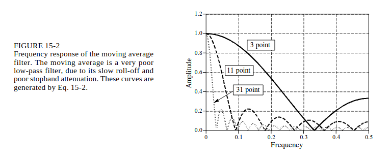
The moving average is the most common filter in DSP, mainly because it is the easiest digital filter to understand and use.

In spite of its simplicity, the moving average filter is optimal for a common task:
reducing random noise while retaining a sharp step response.

This makes it the premier filter for time domain encoded signals.

However, the moving average is the worst filter for frequency domain encoded signals,
with little ability to separate one band of frequencies from another.

Relatives of the moving average filter include the Gaussian, Blackman, and multiple- pass moving average.

These have slightly better performance in the frequency domain, at the expense of increased computation time.

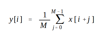
From an implementation view it is convenient that sample frequency has not to be considered and be a part of the filtering algorithm. The filter can be run in realtime on sampled data where the i'th value may be calculated as:

From the litt above:

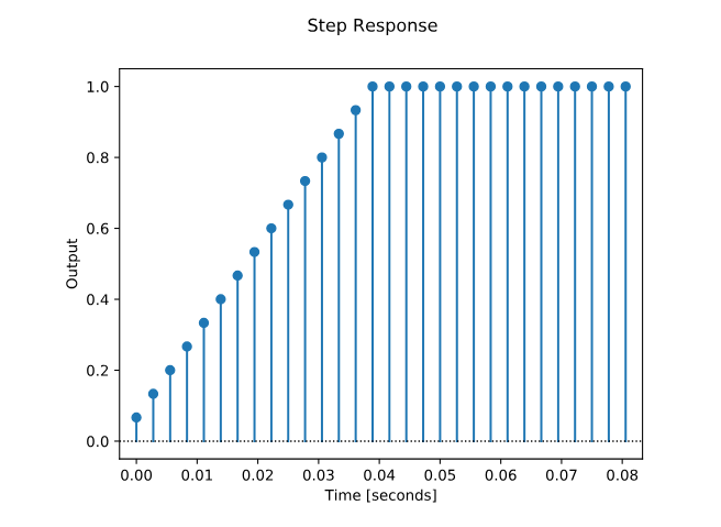
Higher order gives more efficient filtering but do also by nature has an impact on rapid changes like a step response.

From this page the figure below is borrowed where we can see how a stepresponse if flattened out by a 15 sample long averaging filter.

The step response takes 15 samples to stabilize - as predicted.

Still - a moving average filter can with succes be used in many cases and is easy to implement.

Multiple filtering

A way to obtain better filtering is by multiple passes on your data with the SMA algorithm.

The following figures are from https://motorbehaviour.wordpress.com/2011/06/11/moving-average-filters/

Situation

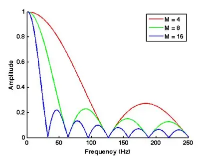
A signal sampled with 500 Hz (X axis is up to 250 Hz : Nyquist criteria)
4,8 and 16 samples long SMA on the signal gives the frequency spectrum as seen on the figure

IN the multipass invariant we can see that using a 8 sample long SMA and apply it several times (1,2,4) you will get the following.

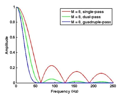Please note the increased damping - also compared with the 16 pins single version above(blue).

Please note it is frequency domain so no info about the delay

An example

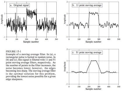
In the figure below a noisy squarewave signal is filtered by a 11 and a 51 point SMA.

The result is

a more clean signal.
The 51 pins SAM reduce more noise than the 11 pins but do alse change shape from square wave to saw alike
In fig you can see a minor deviaion from vertical. In fig c this is much more viewable due to the long SMA.

I would prefere somthing between 11 and 51 pins.

NOTE: that by just looking at the 51 pins it looks like an off line non realtime filtering. This can be seen that from about 180 sample number the 51 pin filtering starts going from 0 to 1 in value. In a(original) we see that it starts going from 0 to 1 at sample nr 200.

So if we are doing SAM in realtime we would in fig c see a delay before the signal starts rinsing about …. 51 samples.

So use as short as possible SMAs

Some code (no guarantee :-)

#define NRPINS 5

int dataAr[NRPINS];

int dataIndex=0;
int dataSum = 0;

void initSMA()
{
	for (int i = 0; i < NRPINS; i++)
	{
		dataAr[i] = 0;
	}
}

int calcSMA(int newSample)
{

	dataSum -= dataAr[dataIndex];
	dataSum += newSample;

	dataAr[dataIndex] = newSample;

	dataIndex++;
	dataIndex %=NRPINS;

	return 	dataSum/NRPINS;
}

int main()
{
	int filterV;
	while (1) {
	// wait on right time to sample

	filterV = calcSMA(readAnalogPort(123));

	// do something :-)
	}
}

For the interested people some links

https://dsp.stackexchange.com/questions/9966/what-is-the-cut-off-frequency-of-a-moving-average-filter
https://motorbehaviour.wordpress.com/2011/06/11/moving-average-filters/
- please note the technique to apply the same filter several times